Unhide the very first column or row of a sheet

Unhide the very first column or row of a sheet

If the first row (Row1) or column (A Column) is hidden in the sheet then un-hiding it could be a bit tricky. The reason is that it’s hard to select that row or column. Though we can select the entire sheet and then unhide rows/columns but that will unhide all columns/rows that we might not want.

Below is an easy way mentioned to do this.

In the Name box which is next to formula bar, write A1 and then press enter button.

Now go to Home tab, in the cells group and Click on Format.

Now under Visibility, click Hide & unhide and then click on unhide rows or unhide columns.

This will unhide the column/row.

Lock Specified Area of a Protected Sheet

Lock Specified Area of a Protected Sheet

When we protect a sheet, all cells are locked by default for editing. For making editable all cells and leaving a few locked, we need to first unlock all cells and then lock specified cells before protecting a sheet.

v  If a sheet is already protected then unprotect it. (Review Tab)

v  Select the whole sheet by Selecting All Button or pressing Ctrl A

v  On the Home tab Click the Format Cells launcher, alternate way is through right click or Ctrl 1.    

v  Got to protection tab and clear the locked check box and click ok. This will unlock all the cells on the sheet, once protected.

v  In your worksheet select only those cells that you want to lock.

v  Again open Format Cells Launcher, same we did earlier.

v  On the protection tab, select the Locked check box and click Ok.

v  Got to Review tab and click Protect Sheet.

v  In the Allow users of this worksheet to list, select the components that we want user to be able to change.

v  In the password to unprotect sheet box, type a password for sheet. Please note the password step is optional, if we don’t provide then any user can unprotect by just clicking on unprotect option.

Viewing two sheets of the same workbook side by side

Viewing two sheets of the same workbook side by side

ü  Go to View tab and in the Window group, click on New Window. This will open a copy of your workbook and also activate the View Side by Side option.

ü  Now click on View Side by Side. (View Tab & Window Group)

ü  Now in a Window you have two views side by side, click the worksheets that you want to compare i.e. sheet1 in first view and sheet2 in second view.

ü  To scroll both worksheets at the same time, click Synchronous Scrolling in the Window group on the View tab.

NOTE: This option is available only when View Side by Side is turned on.

To view two sheets next to each other or in a tiled layout

For this just stay in the View Tab and click on the Arrange All button. This will give multiple display options i.e. Tiles, Horizontal, Vertical & Cascade. Please try the one of your choice.

Interactive Image in Excel

We can make an interactive image in MS Excel. This is explained below step by step.

Interactive Image means, changing of image by changing data of a particular cell.

Suppose If I select or write person A’s name in cell then his/her picture should show up in the corresponding cell and if type the name of Person B then picture should change to of that person.

We will use the options of Camera, Data Validation & Define Name.

We will use the formulas of Vlookup, Indirect & Concatenate.

Add Camera Option to the Quick Access Toolbar

Go to File Menu bas (Excel 2010)

Click Options

Click/Select Quick Access Toolbar from left bar

Choose All Commands from the drop down for Choose Commands form

Select Camera option from the list under All Commands

Now Add the Camera option to the Quick Access Toolbar

Click Ok

Now, we can find the Camera option in the Quick Access Toolbar

Insert/Export the required Images to Excel

We should have the images with us on our system that we want to use in our Excel file. Please follow the below steps to insert images.

Click on Insert Button and then Picture

Locate the Picture one by one and insert in Excel

Re-size the width and height of all the pictures by dragging the edge of image.

The first picture should be in Cell A1 and the second in Cell A2

We need to ensure that image fit in one cell, by setting the column width & row height of the cell.

Rename the sheet as Image.

Now making the Interactive Images

Go to second/next sheet and name it as Interactive Image.

Go to Cell A1

Click on Data tab & then Data Validation.

Select List from the Allow drop down

Type Pizza & Bread in source box & Click OK

Now we have drop won option in Cell A1, select there the first one ‘Pizza’.

In the cell Y1 type Pizza & in Z1 1 and in Cell Y2 Bread & in Z2 2. We will use this data in our formula.

Use shortcut Ctrl+F3 (then name manager box appears)

Click New (then New Name window appears)

Type Name as "Image"

Enter the below formula in the Refers to box 

=INDIRECT("Image!A"&VLOOKUP('Interactive Image'!$A$1,'Interactive Image'!$Y$1:$Z$4,2,0))

Go to Cell C1

Click Camera option from the Quick Access Toolbar (then you get a cross symbol as cursor)

Drop that cross symbol somewhere in the visible Cell (then excel displays image showing G1 Cell content)

Change the formula to =image from =$C$1 (once you select the image you can find the formula in the formula bar)

Now check that changing the Input in Cell A1 (Where Data Validation was done) will change the image that we have placed in/near cell C1.

Deleting Blank rows, a simple technique

Deleting Blank rows, a simple technique

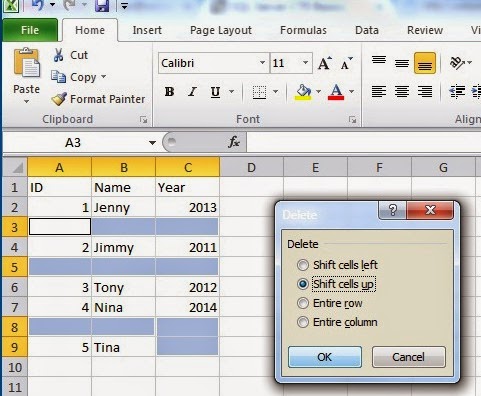
Suppose our data is like below, and we want to delete the blank rows, then no need to do this one by one, use the below technique.

Select the data where in between there are blank rows.

Press F5 button, the below window will appear, now click on Special

Now select the box of Blanks and press ok.

Now blanks are selected so to delete them press Ctrl – and shift the cells up, now data like below.