Check if list of Emails Valid or not (VBA Regex)

If we have a list of email addresses, like about 20,000 and we want to check if they are valid i.e. (valid format with an email id followed by ‘@’ and then domain name) then this macro can help us in doing this with a click.

Example sheet also available at end for Download

We will use VBA and the regular expression function (Regex).

To use Regex we need to do a few things beforehand.

Add VBA reference to "Microsoft VBScript Regular Expressions 5.5"

Ø For this select the “Developer tab”. If you don’t have it then (for Office 2010) go to File -> Options ->Customize Ribbons ->Popular Commands in Choose commands from -> Click on Developer tab box in customize the ribbon box.

Ø Now you can see the Developer tab on top, click on it and then on Visual Basic.

Ø Go to Tools -> References and select Microsoft VBScript Regular Expressions 5.5.




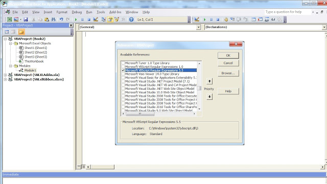
Now you are set to run the Regex Macros.

Below is the VB Code of Macro.

Sub amiq()

Dim strPattern As String: strPattern = "^[\w-\.]{1,}\@([\da-zA-Z-]{1,}\.){1,}[\da-zA-Z-]{2,3}$"
Dim regEx As New RegExp
Dim strInput As String
Dim r As Integer

For r = 2 To Selection.Rows.Count
If strPattern <> "" Then
strInput = Cells(r, 1).Value
With regEx
.Global = True
.MultiLine = True
.IgnoreCase = False
.Pattern = strPattern
End With

If regEx.Test(strInput) Then

Cells(r, 2).Value = "Valid Email Address"
Else
Cells(r, 2).Value = "Not Valid"
End If
End If
Next r
End Sub


I have found this Regex pattern to check mail address validity from totorialspoint.

Please download the example Macro enabled workbook to see how it works. You just need to paste the list of mails in the first column then select and press the button. The second column will show their validity status.


Click Here to Download the Example File

Similarly if we want to identify the cases where text field have consecutive duplicate words and store the duplicate word in results, then we can use the below regex pattern.

Sub amiq()

Dim strPattern As String: strPattern = "\b(\w+)\b\s+\1\b"

Dim regEx As New RegExp

Dim strInput As String

Dim r As Integer

For r = 2 To Selection.Rows.Count

If strPattern <> "" Then

strInput = Cells(r, 6).Value

With regEx

.Global = True

.MultiLine = True

.IgnoreCase = False

.Pattern = strPattern

Set allMatches = regEx.Execute(strInput)

End With

If allMatches.Count <> 0 Then

Cells(r, 7).Value = allMatches.Item(0)

Else

Cells(r, 7).Value = "Valid"

End If

End If

Next r

End Sub

One Drop down List Dependent on Other (Excel 2010)

One Drop down List Dependent on Other

For example in first drop down, we select the type of food, i.e. American or Pakistani. And the second drop down shows us a list of respective food items.

To do this, we need to do the following easy steps.

On the second sheet of our workbook, create named ranges of following.

American	Pakistani	Types
Pizza	Chargha	American
Pasta	Chicken Karahi	Pakistani
Sausage	Naan Cholay

Creating a named range is very easy, for this go to formula tab and click on Define name. If you cursor is in the header row of column the box will pick it. In the “refers to”, add the range excluding the header row.

This way we will create three named ranges.

Now go back to sheet1 and in Column A1 & A2, add labels/heads like Type of Food and Food Item.

Have your cursor in row A2 and go to Data tab and click on Data Validation.

In the Allow box, select list. And in source box refer the named range of Type, like the below snapshot.

Now go to row B2 and, like we did earlier, go to Data tab and click on Data Validation.

In the Allow box, select list. And in source box enter this formula.

=INDIRECT($A$2)

And we are done. Now, the drop down values of second column, are dependent on first one.

Click here to download the example dependent drop down sheet

Gantt Chart in MS Excel 2010

Gantt chart

Note: Recently, I posted a fresh post, along video, on creation of Gantt Chart, which is more simple and easy

http://amiqexcel.blogspot.com/2021/01/gantt-chart-in-ms-excel-urduhindi-just.html

As per Wikipedia, the Gantt chart is a type of bar chart, adapted by Karol Adamiecki in 1896, and independently by Henry Gantt in the 1910s, that illustrates a project schedule. Gantt charts illustrate the start and finish dates of the terminal elements and summary elements of a project.

We can build this chart in Microsoft Excel also. Please see the step by step illustration.

1-      First we should have a list of data i.e. task table to build the chart.

Task	Start Date	Duration	End Date
Brain Storming	5/2	4	5/6
Listing Ideas	5/6	4	5/9
Selecting Idea	5/9	3	5/11
Estimating	5/11	2	5/12
Executing	5/11	2	5/13
Managing	5/12	2	5/14
Reporting	5/13	2	5/12
Meeting	5/13	2	5/12

2-      Make a Bar chart

From the top menu bar, select Insert then Bar and the 2D Stacked Bar. This will inert a blank chart.

3-       Have your mouse in blank Excel chart and click there and then left click -> Select Data. The source window will appear.

Click on legend entries (click add). This will open the series window.

In the series name box, select the cell reference of Start date column header. Like, if our data is in Column A to D, this would be B1.

In the series values box, select the data range of start date column i.e. b2:b9. Click ok and start dates data is in the chart

In same way add the durations.

Now, we will change the dates on the left side to list of tasks.

For this under Horizontal (Category) Axis labels, click on edit.

With mouse highlight the names of tasks and not include the name of column itself i.e A2:A9. Click ok.

Now chart looks like below.

Now Format the Gantt chart

Our task names are in reverse order to correct this, select task names and right click then

Format Axis. And then in Axis options, check the box of categories in reverse order and close.

For more space in chart, select the start date and duration legend/label with mouse and delete them.

Now hide the blue portions of the chart.

Click on any blue bar, this will select all, right click and choose Format Data series.

Ø  Click on Fill then select no fill

Ø  Now click on Border color and select No Line.

We are almost done. We just need to remove the empty extra area from the start.

Go to the first start date cell in the list, in our case it is A2. Now right click and select Format cell. In the Category section, select General. And note the number appearing, in our case it is 42126. Cancel as we are not changing anything, just need this number to use somewhere else.

In the Gantt chart select the dates appearing at top. Click there to select all and then right click and click on Format Axis.

In the Axis options change the minimum bound to the number, we noted.

Change the major unit to 2 and then press Close.

To remove most of the spaces and make the chart look nicer. Click on the top first bar and right click, select Format Data series.

Change the Gap width to 10%

We are finished, our Gantt chart look like this.

Use Mid, Find & Len function to extract substring

Use Mid, Find & Len function to extract substring

Mid function requires three arguments, first the text (could be a cell reference) to look in, the start point and number of characters to return.

What to do when the start position and number of characters to return (length) is unknown?

For example we have a list of email addresses and we want to extract the domain which is after @.

Here comes the use of Find function along Mid function. The Find function, have three arguments. First one is text to find, second is within text (could be a cell reference) and third the starting point of search is optional.

Suppose in cell A2 we have an email address amiqullah@gmail.com . With Find function, we can know the position of @. So the syntax would =FIND("@",A2,1) and the result is 10. So the domain name in this mail address is starting from 11 onward.

Now let us use the Mid function to extract the domain name. Example is given below.

v  The email address is in cell A2. So first specify the text we are looking in =Mid(A2,

v  After that we need to tell the starting point for that use Find function and add 1 so if the Position of @ is 10, we want our search start from 11. FIND("@",A2,1)+1

v  Now the third argument is to specify the length of text that we want to extract. For that first pull the length of our email address len(a2) and then exclude the length of characters that are till @. For that use the same Find function. So complete syntax is LEN(A2)-FIND("@",A2,1).

v  And our complete formula is MID(A2,FIND("@",A2,1)+1,LEN(A2)-FIND("@",A2,1))

In case of any confusion, please feel free to contact me.

A	B	Formula in Cell B
amiqullah@gmail.com	gmail.com	MID(A2,FIND("@",A2,1)+1,LEN(A2)-FIND("@",A2,1))
anjum@shalimar.com	shalimar.com	MID(A3,FIND("@",A3,1)+1,LEN(A3)-FIND("@",A3,1))
nawazanjum@malikgulfaraz.com	malikgulfaraz.com	MID(A4,FIND("@",A4,1)+1,LEN(A4)-FIND("@",A4,1))
Mianamjad@quresh.com	quresh.com	MID(A5,FIND("@",A5,1)+1,LEN(A5)-FIND("@",A5,1))

Use of Excel SIGN Function

SIGN Function

The Excel sign function checks the sign of a number and gives result of 1 if the number is positive, 0 if number is zero and -1 if the number is negative.

Here we have a use of SIGN function. For example we have cost data of this year and last year and we are looking at % variance.

Please see in the below table when value is changing from -18 to -10 the normal calculation give us % change as -44%. Even though there is improvement in year over year number but the % is in negative. So we can use the SIGN function here to return the correct result each time.

A	B	C	D
Cost YE 2014	Cost YE 2015	Variance calculated with Sign function	Variance calculated by normal standard	Formula in Cell C	Formula in Cell D
-18	-10	44%	-44%	(B3-A3)/A3*SIGN(A3)	(B3-A3)/A3
10	12	20%	20%	(B4-A4)/A4*SIGN(A4)	(B4-A4)/A4
13	11	-15%	-15%	(B5-A5)/A5*SIGN(A5)	(B5-A5)/A5
-11	-10	9%	-9%	(B6-A6)/A6*SIGN(A6)	(B6-A6)/A6

Data Validation – Dynamic (Excel 2010) – From Table

Data Validation – Dynamic (Excel 2010) – From Table

Data validation is used so users enter the expected data only, available in a drop down. But with static data validation, if we want to add more values in our list, we will first have to update the source list and then update the source range in Data Validation.  

But there is a way to handle this issue. For example, in column A we have a few product’s listed which we want in another cell to appear in drop down. And as per our need when we add/modify another product in the list (Column A), it start appearing in the drop down.

1- For this, first create a table of the list, for this select the data A1:A9 and press Ctrl T.

2- The default table name is Table1, if you want to change then have your cursor somewhere in the table and go to design tab, under table name the name is appearing and can be changed.

3- Select all record of the table excluding the header (A2:A9) then go to Formulas tab > Define Name and give a name to highlighted range i.e. product

4- In the Refers to tab refer the table like in our case =Table1

5- Select Cell C1 and go to Data > Data Validation. In the Data Validation dialog box, settings tab, choose list under Allow: and in the source box write equal sign and the named range. Like in our example it would be =Product. Press Ok.

6- The drop down list is available in cell C1

7- Now important thing is that we can add a new value to our list, simple go to cell A10 and type another product and press ok or move out of cell and check in C1 cell, the new product is in the list.

Please refer to below snapshots for better idea.

Excel Fill Series

Excel Fill Series

For example, we want to create a list of dates from 01/01/2015 to 12/31/2015. We can type the date 01/01/2015 in cell A1 and then drag it down until we reach 12/31/2015. It will take some time as it’s difficult to stop the mouse at exactly the right cell.

So an option is to use the fill series option. The series dialog box has many options and some of them get automatically selected as the selected cell in our case has a date. If the value in the first cell is a number then we’ll see the ‘Date unit’ options are greyed out:

As we want to fill dates down column A, so we need columns selected.

--Type as Excel detected is Date.

--It has also assumed that we want to increase series by days, as opposed to weekdays, months or years.

--And the step value or increment value is one day at a time.

--So I need to enter the stop value which is last date of my series which in our case is 12/31/2015.

Click ok and you will have a list of dates from January 1 2015 to December 31, 2015 in a few clicks.

Note: (I learned it from http://www.myonlinetraininghub.com/)

Pictograph in Excel

Pictograph in Excel

We can paste a picture from clipboard onto a chart.

For this click on your picture and copy it, suppose it’s in MS Word so copy from there then click on graph series and paste it there (ctrl v).

See the below snap, first graph is standard and the other is with Pic.

We can do some more formatting as well. For that right click on series then Format Data series. Then go to ‘Fill’ Option. There are 3 options. Stretch is default, Stack and Stack & Scale to.

With Stack option the chart will look like below.

With Stack & scale option, we can enter input.

There are other options in the Fill tab like Gradient Fill, Picture or texture fill, which can be tried to make bars look more eye catching.

Using “Playbill” font & Excel formula for incell charts

Using “Playbill” font & Excel formula for incell charts

With REPT formula and symbol (“|”), we can make in-cell charts. And to look them just like a chart, use the playbill font. We can change the theme color as well to make it more prominent/attractive.

For example, our data is in range D3:D7. Use the below formula. Here we are repeating the symbol and the number of times is the cell value divided by the maximum number of the list/range and multiplied by hundred. It’s easy & simple, just try it.

=REPT("|",D3/MAX($D$3:$D$7)*100)

Excel formula: COUNTIFS() with date range in cell reference

Excel formula: COUNTIFS() with date range in cell reference

Suppose we have soma data with dates and we want to count the rows, falling between two dates.  I had to do the same thing today and faced an issue. Though most of the people would be already aware of it but for a person like me, it was a new thing so thought to share with everyone.

If we do the date comparison this way “>=G1”, here G1 is the cell where start date is written then this check will not work. Though, it will work, if we specify a date itself instead of cell reference. For cell reference, the comparison operator will be in double quotes and with & we will add the cell reference. Please see the complete syntax. Here the B:B is the column range/criteria range having dates and G1 & H1 are start & end dates.

=COUNTIFS(B:B,">="&G1,B:B,"<="&H1)

Power Pivot Table (Excel 2010)

Power Pivot is a free add-in to the 2010 version and can be downloaded from below link. It comes with Office 2013 Pro & Office 365.

Download Link: https://support.office.com/en-nz/article/Power-Pivot-Add-in-a9c2c6e2-cc49-4976-a7d7-40896795d045

Power Pivot extends capabilities of the pivot data summarization and we can import data from multiple data sources.

The following free Microsoft Virtual Academy course can be very helpful in learning Power Query & Power Pivot along more info.

http://www.microsoftvirtualacademy.com/training-courses/faster-insights-to-data-with-power-bi-jump-start

In this post, I will share a basic use of Power Pivot with example in Excel 2010.

Once we have downloaded the add-in, we would be able to see it in our workbook in top ribbon.

With Power Pivot, we can link our multiple tables through the common Key/Column between them. It’s just like the relational database. Once we have linked them, then they could be summarized at one place. We will see it in this post step by step.

We have the below 3 tables of data in the 3 separate sheets.

Customer Table

KeyCustomer	Name	Gender	Type	State/Province
306256	Mary	Female	Individual	Punjab
306257	Sally	Female	Individual	Sindh
306258	Asif	Male	Individual	KPK
306259	Arif	Male	Individual	Punjab
306260	Nadeem	Male	Individual	Sindh
306261	William	Male	Company	KPK
306262	Michael	Male	Company	Punjab
306263	Natasha	Female	Individual	Sindh
306264	Praveen	Female	Individual	KPK
306265	Nazar	Male	Company	Punjab

Product Table

ProductKey	P-Name	Price	Size
P-123	T-Shirt	350	Large
P-124	T-Shirt	300	Medium
P-125	T-Shirt	250	Small
P-126	Hockey Stick	800	Large
P-127	Hockey Stick	750	Medium
P-128	Hockey Stick	700	Small
P-129	Tennis Racket	1000	Large
P-130	Tennis Racket	950	Medium
P-131	Tennis Racket	800	Small
P-132	Bag	1000	Large
P-133	Bag	950	Medium
P-134	Bag	800	Small

Sales Table

SalesID	Date	KeyCustomer	ProductKey	Quantity
S-111	12/1/2014	306256	P-123	2
S-112	12/1/2014	306257	P-124	3
S-111	12/1/2014	306258	P-125	1
S-112	12/1/2014	306259	P-126	4
S-111	12/1/2014	306260	P-127	5
S-112	12/1/2014	306261	P-128	3
S-111	12/1/2014	306262	P-129	2
S-112	12/2/2014	306263	P-130	6
S-111	12/2/2014	306264	P-131	9
S-112	12/2/2014	306265	P-132	1
S-111	12/3/2014	306261	P-133	2
S-112	12/10/2014	306262	P-134	2
S-111	12/15/2014	306263	P-126	2
S-112	12/16/2014	306261	P-127	3
S-111	12/17/2014	306262	P-128	1
S-112	12/18/2014	306263	P-129	4
S-111	12/19/2014	306265	P-131	5
S-112	12/20/2014	306261	P-132	3
S-111	12/21/2014	306262	P-133	2
S-112	12/22/2014	306263	P-131	6
S-111	12/23/2014	306261	P-132	9
S-112	12/24/2014	306262	P-133	1
S-111	12/25/2014	306263	P-133	2
S-112	12/26/2014	306259	P-134	2
S-111	12/27/2014	306260	P-125	2
S-112	12/28/2014	306261	P-126	3
S-111	12/29/2014	306262	P-127	1
S-112	12/30/2014	306263	P-134	4
S-111	12/31/2014	306264	P-126	5
S-112	1/1/2015	306265	P-127	3

Have your data in table form, for this select your data and press CtrlL. Name your table, just for clarity. For this have your cursor somewhere in table and go to design tab and change the default table name there.

After that click on the PowerPivot which would be at the top bar. Your cursor be in somewhere the table i.e Customer Table and then click on Create Linked Table. This will move the table in Power Pivot window. Do this for all the tables and move the 3 tables.

Now Go to Design Tab in Power Pivot window and then click on Create Relationship, a new window will open.

Relate the Product and Sales table on ProductKey Column and Customer and Sales Table on KeyCustomer Column, one by one.

This way all the three tables are linked now.

For any change in relationship click on Manage Relationship

To view the Diagram View of relationships, go to Table Tools tab and then click on Diagram View.

Once the relationship is finalized, go to workbook, PowerPivot then PivotTable and Create Pivot table as we do, but here we can have data from all the 3 tables in our Pivot table.